Background

The chain rule, gradient (Jacobian), computational graph, elementary functions and several numerical methods serve as the mathematical cornerstone for this software. The mathematical concepts here come from CS 207 Lectures 9 and 10 on Autodifferentiation.

The Chain Rule

The chain rule is critical to AD, since the derivative of the function with respect to the input is dependent upon the derivative of each trace in the evaluation with respect to the input.

If we have \(h(u(x))\) then the derivative of \(h\) with respect to \(x\) is:

\[\frac{\partial h}{\partial x} =\frac{\partial h}{\partial u} \cdot \frac{\partial u}{\partial x}\]

If we have another argument \(h(u, v)\) where \(u\) and \(v\) are both functions of \(x\), then the derivative of \(h(x)\) with respect to \(x\) is:

\[\frac{\partial h}{\partial x} =\frac{\partial h}{\partial u} \cdot \frac{\partial u}{\partial x} + \frac{\partial h}{\partial v} \cdot \frac{\partial v}{\partial x}\]

Gradient and Jacobian

If we have \(x\in\mathbb{R}^{m}\) and function \(h\left(u\left(x\right),v\left(x\right)\right)\), we want to calculate the gradient of \(h\) with respect to \(x\):

\[\nabla_{x} h = \frac{\partial h}{\partial u}\nabla_x u + \frac{\partial h}{\partial v} \nabla_x v\]

In the case where we have a function \(h(x): \mathbb{R}^m \rightarrow \mathbb{R}^n\), we write the Jacobian matrix as follows, allowing us to store the gradient of each output with respect to each input.

\[\begin{split}J = \begin{bmatrix} \frac{\partial h_1}{\partial x_1} & \frac{\partial h_1}{\partial x_2} & \ldots & \frac{\partial h_1}{\partial x_m} \\[1ex] \frac{\partial h_2}{\partial x_1} & \frac{\partial h_2}{\partial x_2} & \ldots & \frac{\partial h_2}{\partial x_m} \\[1ex] \vdots & \vdots & \ddots & \vdots \\[1ex] \frac{\partial h_n}{\partial x_1} & \frac{\partial h_n}{\partial x_2} & \ldots & \frac{\partial h_n}{\partial x_m} \end{bmatrix}\end{split}\]

In general, if we have a function \(g\left(y\left(x\right)\right)\) where \(y\in\mathbb{R}^{n}\) and \(x\in\mathbb{R}^{m}\). Then \(g\) is a function of possibly \(n\) other functions, each of which can be a function of \(m\) variables. The gradient of \(g\) is now given by

\[\nabla_{x}g = \sum_{i=1}^{n}{\frac{\partial g}{\partial y_{i}}\nabla_x y_{i}\left(x\right)}.\]

The Computational Graph

Let us visualize what happens during the evaluation trace. The following example is based on Lectures 9 and 10. Consider the function:

\[f\left(x\right) = x - \exp\left(-2\sin^{2}\left(4x\right)\right)\]

If we want to evaluate \(f\) at the point \(x\), we construct a graph where the input value is \(x\) and the output is \(y\). Each input variable is a node, and each subsequent operation of the execution trace applies an operation to one or more previous nodes (and creates a node for constants when applicable).

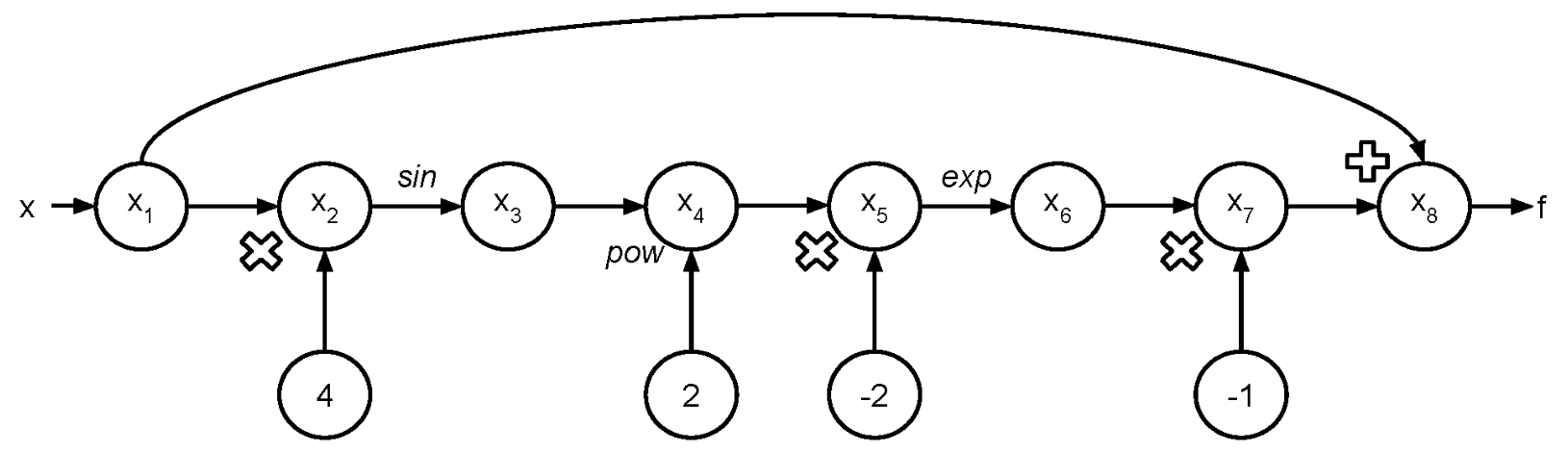
As we execute \(f(x)\) in the “forward mode”, we can propagate not only the sequential evaluations of operations in the graph given previous nodes, but also the derivatives using the chain rule.

Elementary functions

An elementary function is built up of a finite combination of constant functions, field operations \((+, -, \times, \div)\), algebraic, exponential, trigonometric, hyperbolic and logarithmic functions and their inverses under repeated compositions. Below is a table of some elementary functions and examples that we will include in our implementation.

Elementary Functions	Example
powers	\(x^2\)
roots	\(\sqrt{x}\)
exponentials	\(e^{x}\)
logarithms	\(\log(x)\)
trigonometrics	\(\sin(x)\)
inverse trigonometrics	\(\arcsin(x)\)
hyperbolics	\(\sinh(x)\)

Note

Background for additional features, Newton’s root finding, Gradient Descent, BFGS and quadratic splines can be found in Additional Features.