Additional Features
Root finding
Background
Newton root finding starts from an initial guess for \(x_1\) and converges to \(x\) such that \(f(x) = 0\). The algorithm is iterative. At each step \(t\), the algorithm finds a line (or plane, in higher dimensions) that is tangent to \(f\) at \(x_t\). The new guess for \(x_{t+1}\) is where the tangent line crosses the \(x\)-axis. This generalizes to \(m\) dimensions.
- Algorithm (univariate case)
- for \(t\) iterations or until step size <
tol: - \(x_{t+1} \leftarrow x_{t} - \frac{f(x_t)}{f'(x_t)}\)
- Algorithm (multivariate case)
- for \(t\) iterations or until step size <
tol: - \(\textbf{x}_{t+1} \leftarrow \textbf{x}_t - (J(f)(\textbf{x}_t))^{-1}f(\textbf{x}_t)\)
In the multivariate case, \(J(f)\) is the Jacobian of \(f\). If \(J(f)\) is non-square, we use the pseudoinverse.
Here is an example in the univariate case:
A common application of root finding is in Lagrangian optimization. For example, consider the Lagrangian \(\mathcal{L}(\textbf{b}, \lambda)\). One can solve for the weights \(\textbf{b}, \lambda\) such that \(\frac{\partial \mathcal{L}}{\partial b_j} = \frac{\partial \mathcal{L}}{\partial \lambda} = 0\).
Implementation
Methods
NewtonRoot: return a root of a function \(f: \mathbb{R}^m \Rightarrow \mathbb{R}^1\)input:
f: function of interest, callable. If \(f\) is a scalar to scalar function, then define \(f\) as follows:1 2 3
def f(x): # Use x in function return x ** 2 + np.exp(x)
If \(f\) is a function of multiple scalars (i.e. \(\mathbb{R}^m \Rightarrow \mathbb{R}^1\)), the arguments to \(f\) must be passed in as a list. In this case, define \(f\) as follows:
1
2
3
def f(variables): x, y, z = variables return x ** 2 + y ** 2 + z ** 2 + np.sin(x)
x: int, float, or da.Var (univariate), or list of int, float, or da.Var objects (multivariate). Inital guess for a root of \(f\). If \(f\) is a scalar to scalar function (i.e. \(\mathbb{R}^1 \Rightarrow \mathbb{R}^1)\), and the initial guess for the root is 1, then x = [da.Var(1)]. If \(f\) is a function of multiple scalars, with initial guess for the root as (1, 2, 3), then the user can definexas:1
x = [1, 2, 3]
iters: int, optional, default=2000. The maximum number of iterations to run the Newton root finding algorithm. The algorithm will run for min \((t, iters)\) iterations, where \(t\) is the number of steps untiltolis satisfied.tol: int or float, optional, default=1e-10. If the size of the update step (L2 norm in the case of \(\mathbb{R}^m \Rightarrow \mathbb{R}^1)\) is smaller thantol, then the algorithm will add that step and then terminate, even if the number of iterations has not reachediters.
return:
root: da.Var \(\in \mathbb{R}^m\). The val attribute contains a numpy array of the root that the algorithm found in \(min(iters, t)\) iterations (\(iters, t\) defined above). The der attribute contains the Jacobian value at the specified root.var_path: a numpy array (\(\mathbb{R}^{n \times m}\)), where \(n = min(iters, t)\) is the number of steps of the algorithm and \(m\) if the dimension of the root, where rows of the array are steps taken in consecutive order.g_path: a numpy array (\(\mathbb{R}^{n \times 1}\)), containing the consecutive steps of the output of \(f\) at each guess invar_path.
External dependencies
DeriveAliveNumPymatplotlib.pyplot
Demo
>>> from DeriveAlive import rootfinding as rf
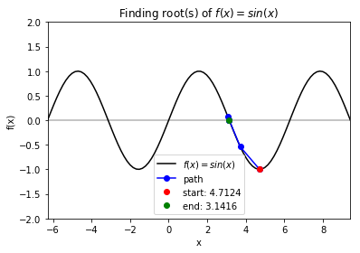
Case 1: \(f = sin(x)\) with starting point \(x_0= \frac{3\pi}{2}\). Note: Newton method is not guaranteed to converge when \(f\prime(x_0)= 0\). In our case, if the current guess has derivative of 0, we randomly set the derivative to be \(\pm1\) and move in that directino to avoid getting stuck and avoid calculating an update step that has an extreme magnitude (which would occur if the derivative is very close to 0).
# define f function
>>> f_string = 'f(x) = sin(x)'
>>> def f(x):
return np.sin(x)
>>> # Start at 3*pi/2
>>> x0 = 3 * np.pi / 2
# finding the root
>>> for val in [np.pi - 0.25, np.pi, 1.5 * np.pi, 2 * np.pi - 0.25, 2 * np.pi + 0.25]:
solution, x_path, y_path = rf.NewtonRoot(f, x0)
# visualize the trace
>>> x_lims = -2 * np.pi, 3 * np.pi
>>> y_lims = -2, 2
>>> rf.plot_results(f, x_path, y_path, f_string, x_lims, y_lims)
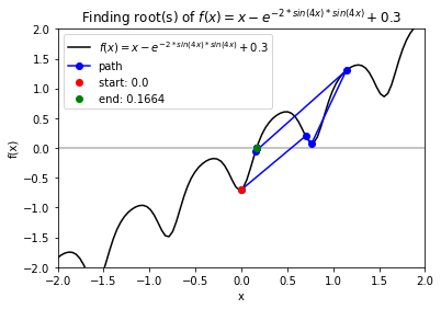
Case 2: \(f = x - \exp(-2\sin(4x)sin(4x)+0.3\) with starting point \(x_0 = 0\).
# define f function
f_string = 'f(x) = x - e^{-2 * sin(4x) * sin(4x)} + 0.3'
>>> def f(x):
return x - np.exp(-2.0 * np.sin(4.0 * x) * np.sin(4.0 * x)) + 0.3
# start at 0
>>> x0 = 0
# finding the root
>>> for val in np.arange(-0.75, 0.8, 0.25):
solution, x_path, y_path = rf.NewtonRoot(f, x0)
# visualize the trace
>>> x_lims = -2, 2
>>> y_lims = -2, 2
>>> rf.plot_results(f, x_path, y_path, f_string, x_lims, y_lims)
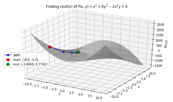
Case 3: \(f(x, y) = x^2 + 4y^2-2x^2y +4\) with starting points \(x_0 =-8.0, y_0 = -5.0\).
# define f function
>>> f_string = 'f(x, y) = x^2 + 4y^2 -2x^2y + 4'
>>> def f(variables):
x, y = variables
return x ** 2 + 4 * y ** 2 - 2 * (x ** 2) * y + 4
# start at x0=−8.0,y0= −5
>>> x0 = -8.0
>>> y0 = -5.0
>>> init_vars = [x0, y0]
# finding the root and visualize the trace
>>> solution, xy_path, f_path = rf.NewtonRoot(f, init_vars)
>>> rf.plot_results(f, xy_path, f_path, f_string, threedim=True)
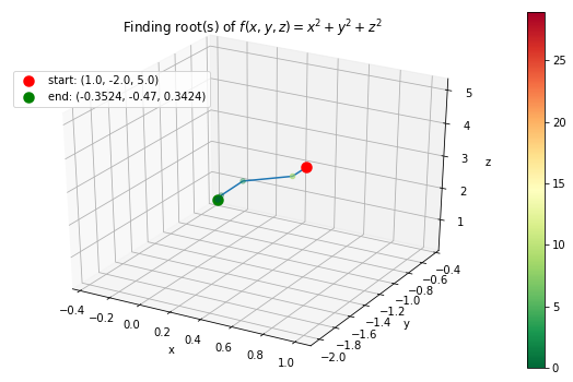
Case 4: \(f(x, y, z) = x^2 + y^2 + z^2\) with starting points \(x_0 =1, y_0 = -2, z_0 = 5\).
# define f function
>>> f_string = 'f(x, y, z) = x^2 + y^2 + z^2'
>>> def f(variables):
x, y, z = variables
return x ** 2 + y ** 2 + z ** 2 + np.sin(x) + np.sin(y) + np.sin(z)
# start at
>>> x0= 1
>>> y0= -2
>>> z0= 5
>>> init_vars = [x0, y0, z0]
# finding the root and visualize the trace
>>> solution, xyz_path, f_path = rf.NewtonRoot(f, init_vars)
>>> m = len(solution.val)
>>> rf.plot_results(f, xyz_path, f_path, f_string, fourdim=True)
Optimization
Background
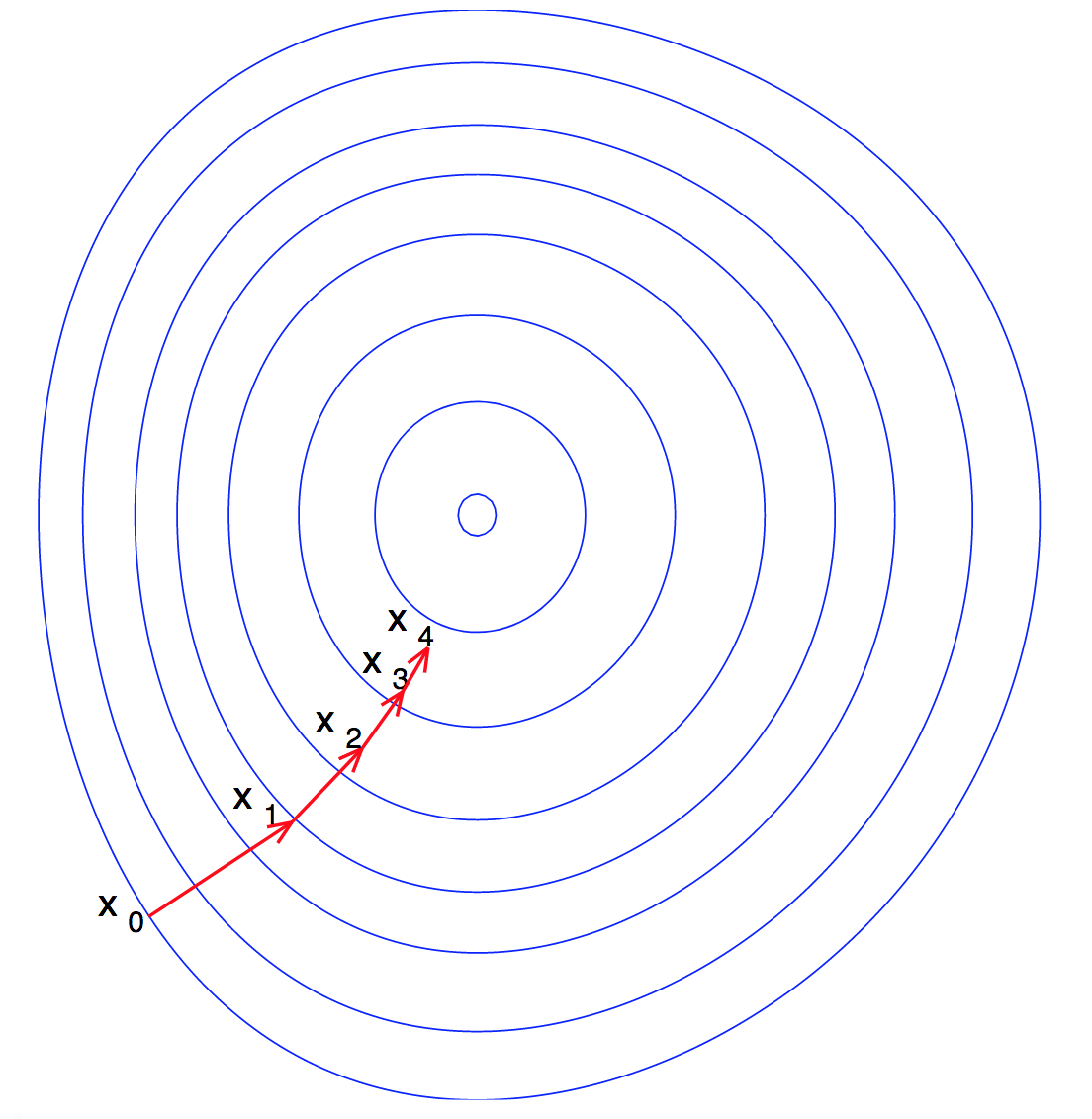
Gradient Descent is used to find the local minimum of a function \(f\) by taking locally optimum steps in the direction of steepest descent. A common application is in machine learning when a user desires to find optimal weights to minimize a loss function.
Here is a visualization of Gradient Descent on a convex function of 2 variables:
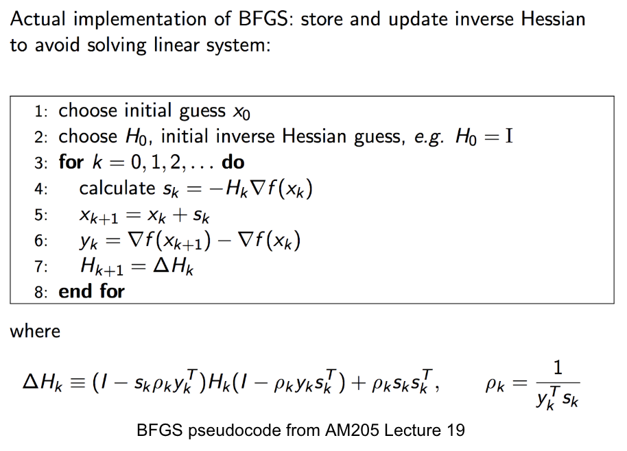
BFGS, short for “Broyden–Fletcher–Goldfarb–Shanno algorithm”, seeks a stationary point of a function, i.e. where the gradient is zero. In quasi-Newton methods, the Hessian matrix of second derivatives is not computed. Instead, the Hessian matrix is approximated using updates specified by gradient evaluations (or approximate gradient evaluations).
Here is a pseudocode of the implementation of BFGS.
Implementation
Methods
GradientDescent: solve for a local minimum of a function \(f: \mathbb{R}^m \Rightarrow \mathbb{R}^1\). If \(f\) is a convex function, then the local minimum is a global minimum.input:
f: function of interest, callable. In machine learning applications, this should be the cost function. For example, if solving for optimal weights to minimize a cost function \(f\), then \(f\) can be defined as \(\frac{1}{2m}\) times the sum of \(m\) squared residuals.If \(f\) is a scalar to scalar function, then define \(f\) as follows:
1 2 3
def f(x):
    # Use x in function
    return x ** 2 + np.exp(x)
If \(f\) is a function of multiple scalars (i.e. \(\mathbb{R}^m \Rightarrow \mathbb{R}^1\)), the arguments to \(f\) must be passed in as a list. In this case, define \(f\) as follows:
1
2
3
def def f(variables):
    x, y, z = variables
    return x ** 2 + y ** 2 + z ** 2 + np.sin(x)
x: int, float, or da.Var (univariate), or list of int, float, or da.Var objects (multivariate). Initial guess for a root of \(f\). If \(f\) is a scalar to scalar function (i.e. \(\mathbb{R}^1 \Rightarrow \mathbb{R}^1)\), and the initial guess for the root is 1, then a valid x is x = 1. If \(f\) is a function of multiple scalars, with initial guess for the root as (1, 2, 3), then a valid definition ofxis as follows:iters: int, optional, default=2000. The maximum number of iterations to run the Newton root finding algorithm. The algorithm will run for min \((t, iters)\) iterations, where \(t\) is the number of steps untiltolis satisfied.tol: int or float, optional, default=1e-10. If the size of the update step (L2 norm in the case of \(\mathbb{R}^m \Rightarrow \mathbb{R}^1)\) is smaller thantol, then the algorithm will add that step and then terminate, even if the number of iterations has not reachediters.
return:
minimum: da.Var \(\in \mathbb{R}^m\). The val attribute contains a numpy array of the minimum that the algorithm found in \(min(iters, t)\) iterations (\(iters, t\) defined above). The der attribute contains the Jacobian value at the specified root.var_path: a numpy array (\(\mathbb{R}^{n \times m}\)), where \(n = min(iters, t)\) is the number of steps of the algorithm and \(m\) if the dimension of the minimum, where rows of the array are steps taken in consecutive order.g_path: a numpy array (\(\mathbb{R}^{n \times 1}\)), containing the consecutive steps of the output of \(f\) at each guess invar_path.
External dependencies
DeriveAliveNumPymatplotlib.pyplot
Demo
>>> import DeriveAlive.optimize as opt
>>> import numpy as np
>>> import matplotlib.pyplot as plt
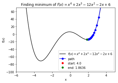
Case 1: Minimize quartic function \(f(x) = x^4\). Get stuck in local minimum.
>>> def f(x):
        return x ** 4 + 2 * (x ** 3) - 12 * (x ** 2) - 2 * x + 6

    # Function string to include in plot
>>> f_string = 'f(x) = x^4 + 2x^3 -12x^2 -2x + 6'

>>> x0 = 4
>>> solution, xy_path, f_path = opt.GradientDescent(f, x0, iters=1000, eta=0.002)
>>> opt.plot_results(f, xy_path, f_path, f_string, x_lims=(-6, 5), y_lims=(-100, 70))
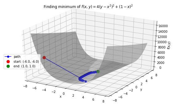
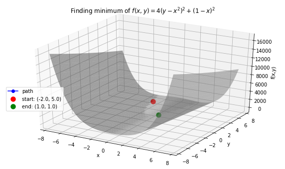
Case 2: Minimize Rosenbrock’s function \(f(x, y) = 4(y - x^2)^2 + (1 - x)^2\). Global minimum: 0 at \((x,y)=(1, 1)\).
# Rosenbrock function with leading coefficient of 4
>>> def f(variables):
        x, y = variables
        return 4 * (y - (x ** 2)) ** 2 + (1 - x) ** 2

# Function string to include in plot
>>> f_string = 'f(x, y) = 4(y - x^2)^2 + (1 - x)^2'

>>> x_val, y_val = -6, -6
>>> init_vars = [x_val, y_val]
>>> solution, xy_path, f_path = opt.GradientDescent(f, init_vars, iters=25000, eta=0.002)
>>> opt.plot_results(f, xy_path, f_path, f_string, x_lims=(-7.5, 7.5), threedim=True)
>>> x_val, y_val = -2, 5
>>> init_vars = [x_val, y_val]
>>> solution, xy_path, f_path = opt.GradientDescent(f, init_vars, iters=25000, eta=0.002)
>>> opt.plot_results(f, xy_path, f_path, f_string, x_lims=(-7.5, 7.5), threedim=True)
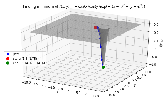
Case 3: Minimize Easom’s function: \(f(x, y) = -\cos(x)\cos(y)\exp(-((x - \pi)^2 + (y - \pi)^2))\). Global minimum: -1 at \((x,y)=(\pi, \pi)\).
# Easom's function
>>> def f(variables):
        x, y = variables
        return -np.cos(x) * np.cos(y) * np.exp(-((x - np.pi) ** 2 + (y - np.pi) ** 2))

# Function string to include in plot
>>> f_string = 'f(x, y) = -\cos(x)\cos(y)\exp(-((x-\pi)^2 + (y-\pi)^2))'

# Initial guess
>>> x0 = 1.5
>>> y0 = 1.75
>>> init_vars = [x0, y0]

# Visulaize gradient descent
solution, xy_path, f_path = opt.GradientDescent(f, init_vars, iters=10000, eta=0.3)
opt.plot_results(f, xy_path, f_path, f_string, threedim=True)
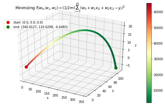
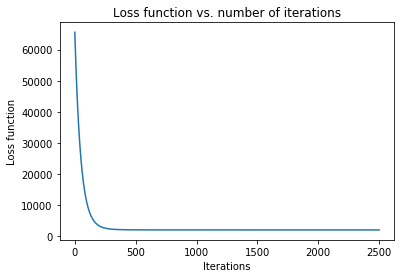
Case 4: Machine Learning application: minimize mean squared error in regression
where \(\textbf{w}\) contains an extra dimension to fit the intercept of the features. - Example dataset (standardized): 47 homes from Portland, Oregon. Features: area (square feet), number of bedrooms. Output: price (in thousands of dollars).
>>> f = "mse"
>>> init_vars = [0, 0, 0]

# Function string to include in plot
>>> f_string = 'f(w_0, w_1, w_2) = (1/2m)\sum_{i=0}^m (w_0 + w_1x_{i1} + w_2x_{i2} - y_i)^2'

# Visulaize gradient descent
>>> solution, w_path, f_path, f = opt.GradientDescent(f, init_vars, iters=2500, data=data)
>>> print ("Gradient descent optimized weights:\n{}".format(solution.val))
>>> opt.plot_results(f, w_path, f_path, f_string, x_lims=(-7.5, 7.5), fourdim=True)
Gradient descent optimized weights:
[340.41265957 110.62984204  -6.64826603]
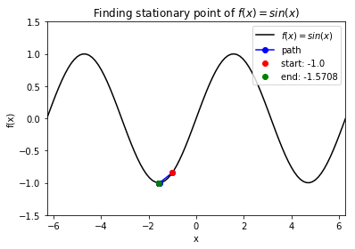
Case 5: Find stationary point of \(f(x) = \sin(x)\). Note: BFGS finds stationary point, which can be maximum, not minimum.
>>> def f(x):
        return np.sin(x)

>>> f_string = 'f(x) = sin(x)'

>>> x0 = -1
>>> solution, x_path, f_path = opt.BFGS(f, x0)
>>> anim = opt.plot_results(f, x_path, f_path, f_string, x_lims=(-2 * np.pi, 2 * np.pi), y_lims=(-1.5, 1.5), bfgs=True)
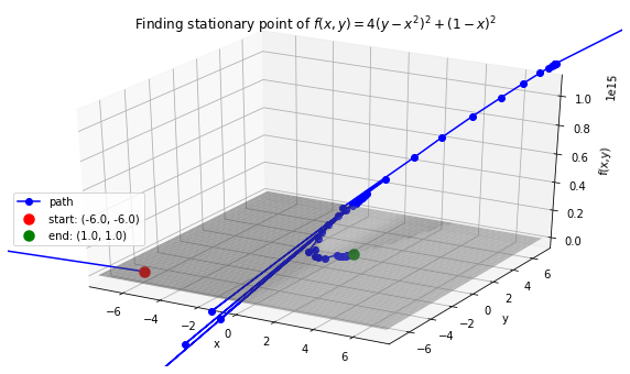
Case 6: Find stationary point of Rosenbrock function: \(f(x, y) = 4(y - x^2)^2 + (1 - x)^2\). Stationary point: 0 at \((x,y)=(1, 1)\).
>>> def f(variables):
        x, y = variables
        return 4 * (y - (x ** 2)) ** 2 + (1 - x) ** 2

>>> f_string = 'f(x, y) = 4(y - x^2)^2 + (1 - x)^2'

>>> x0, y0 = -6, -6
>>> init_vars = [x0, y0]
>>> solution, xy_path, f_path = opt.BFGS(f, init_vars, iters=25000)
>>> xn, yn = solution.val
>>> anim = opt.plot_results(f, xy_path, f_path, f_string, x_lims=(-7.5, 7.5), y_lims=(-7.5, 7.5), threedim=True, bfgs=True)
Quadratic Splines
Background
DeriveAlive package can be used to calculate quadratic splines
since it automatically returns the first derivative of a function at a
given point.- Each \(s_k(x)\) should match the function values at both of its endpoints, so that \(s_k(kh)=f(kh)\) and \(s_k( (k+1)h) =f( (k+1)h)\). (Provides \(2N\) constraints.)
- At each interior boundary, the spline should be differentiable, so that \(s_{k-1}(kh)= s_k(kh)\) for \(k=1,\ldots,N-1\). (Provides \(N-1\) constraints.)
- Since \(f'(x+1)=10f'(x)\), let \(s'_{N-1}(1) = 10s'_0(0)\). (Provides \(1\) constraint.)
Since there are \(3N\) constraints for \(3N\) degrees of freedom, there is a unique solution.
Implementation
- Methods
quad_spline_coeff: calculate the coefficients of quadratic splines- input:
f: function of interestxMin: left endpoint of the \(x\) intervalxMax: right endpoint of the \(x\) intervalnIntervals: number of intervals that you want to slice the original function
- return:
y: the right hand side of \(Ax=y\)A: the sqaure matrix in the left hand side of \(Ax=y\)coeffs: coefficients of \(a_i, b_i, c_i\)ks: points of interest in the \(x\) interval asDeriveAliveobjects
- input:
spline_points: get the coordinates of points on the corresponding splines- input:
f: function of interestcoeffs: coefficients of \(a_i, b_i, c_i\)ks: points of interest in the \(x\) interval asDeriveAliveobjectsnSplinePoints: number of points to draw each spline
- return:
spline_points: a list of spline points \((x,y)\) on each \(s_i\)
- input:
quad_spline_plot: plot the original function and the corresponding splines- input:
f: function of interestcoeffs: coefficients of \(a_i, b_i, c_i\)ks: points of interest in the \(x\) interval asDeriveAliveobjectsnSplinePoints: number of points to draw each spline
- return:
fig: the plot of \(f(x)\) and splines
- input:
spline_error: calculate the average absolute error of the spline and the original function at one point- input:
f: function of interestspline_points: a list of spline points \((x,y)\) on each \(s_i\)
- return:
error: average absolute error of the spline and the original function on one given interval
- input:
- External dependencies
DeriveAliveNumPymatplotlib.pyplot
Demo
>>> import DeriveAlive.spline as sp
>>> import numpy as np
>>> import matplotlib.pyplot as plt
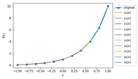
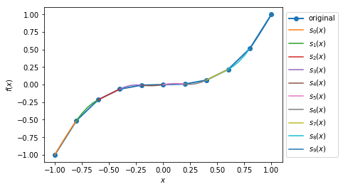
Case 1: Plot the quadratic spline of \(f_1(x) = 10^x, x \in [-1, 1]\) with 10 intervals.
>>> def f1(var):
        return 10**var

>>> xMin1 = -1
>>> xMax1 = 1
>>> nIntervals1 = 10
>>> nSplinePoints1 = 5

>>> y1, A1, coeffs1, ks1 = sp.quad_spline_coeff(f1, xMin1, xMax1, nIntervals1)
>>> fig1 = sp.quad_spline_plot(f1, coeffs1, ks1, nSplinePoints1)
>>> spline_points1 = sp.spline_points(f1, coeffs1, ks1, nSplinePoints1)
>>> sp.spline_error(f1, spline_points1)
0.0038642295476342416

>>> fig1
Case 2: Plot the quadratic spline of \(f_2(x) = x^3, x \in [-1, 1]\) with 10 intervals.
>>> def f2(var):
        return var**3

>>> xMin2 = -1
>>> xMax2 = 1
>>> nIntervals2 = 10
>>> nSplinePoints2 = 5

>>> y2, A2, coeffs2, ks2 = sp.quad_spline_coeff(f2, xMin2, xMax2, nIntervals2)
>>> fig2 = sp.quad_spline_plot(f2, coeffs2, ks2, nSplinePoints2)
>>> spline_points2 = sp.spline_points(f2, coeffs2, ks2, nSplinePoints2)
>>> sp.spline_error(f2, spline_points2)
0.0074670329670330216

>>> fig2
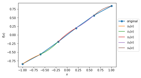
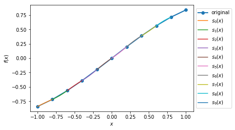
Case 3: Plot the quadratic spline of \(f_3(x) = \sin(x), x \in [-1,1]\) and \(x \in [-\pi, \pi]\) with 5 intervals and 10 intervals.
>>> def f3(var):
        return np.sin(var)

>>> xMin3 = -1
>>> xMax3 = 1
>>> nIntervals3 = 5
>>> nSplinePoints3 = 5

>>> y3, A3, coeffs3, ks3 = sp.quad_spline_coeff(f3, xMin3, xMax3, nIntervals3)
>>> fig3 = sp.quad_spline_plot(f3, coeffs3, ks3, nSplinePoints3)
>>> spline_points3 = sp.spline_points(f3, coeffs3, ks3, nSplinePoints3)
>>> sp.spline_error(f3, spline_points3)
0.015578205778177232

>>> fig3
>>> xMin4 = -1
>>> xMax4 = 1
>>> nIntervals4 = 10
>>> nSplinePoints4 = 5

>>> y4, A4, coeffs4, ks4 = sp.quad_spline_coeff(f3, xMin4, xMax4, nIntervals4)
>>> fig4 = sp.quad_spline_plot(f3, coeffs4, ks4, nSplinePoints4)
>>> spline_points4 = sp.spline_points(f3, coeffs4, ks4, nSplinePoints4)
>>> sp.spline_error(f3, spline_points4)
0.0034954287455489196

>>> fig4
Note
We can see that the quadratic splines do not work that well with linear-ish functions. While adding more intervals may help to make the approximated splines better.
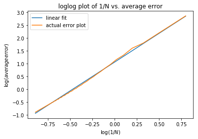
Casee 4: Here we demonstrate that the more intervals will make the splines approximations better using a \(log-log\) plot of the absolute average error with respect to :math: frac{1}{N}` with \(f(x) = 10^x, x \in [-\pi, \pi]\) at intervals from 5 to 100.
>>> def f(var):
        return 10 ** var

>>> xMin = -sp.np.pi
>>> xMax = sp.np.pi
>>> nIntervalsList = sp.np.arange(1, 50, 1)
>>> nSplinePoints = 10
>>> squaredErrorList = []

>>> for nIntervals in nIntervalsList:
        y, A, coeffs, ks = sp.quad_spline_coeff(f, xMin, xMax, nIntervals)
        spline_points = sp.spline_points(f, coeffs, ks, nSplinePoints)
        error = sp.spline_error(f, spline_points)
        squaredErrorList.append(error)

>>> plt.figure()

>>> coefficients = np.polyfit(np.log10(2*np.pi/nIntervalsList), np.log10(squaredErrorList), 1)
>>> polynomial = np.poly1d(coefficients)
>>> ys = polynomial(np.log10(2*np.pi/nIntervalsList))
>>> plt.plot(np.log10(2*np.pi/nIntervalsList), ys, label='linear fit')
>>> plt.plot(np.log10(2*np.pi/nIntervalsList), np.log10(squaredErrorList), label='actual error plot')
>>> plt.xlabel(r'$\log(1/N)$')
>>> plt.ylabel(r'$\log(average error)$')
>>> plt.legend()
>>> plt.title('loglog plot of 1/N vs. average error')
>>> plt.show()
>>> beta, alpha = coefficients[0], 10**coefficients[1]
>>> beta, alpha
(2.2462166565957835, 11.414027075895813)
Note
We can see in the \(log-log\) plot that the log of absolute average error is proportional to the log of \(\frac{1}{N}\), i.e. \(E_{1/N} \approx 11.4(\dfrac{1}{N})^{2.25}\).
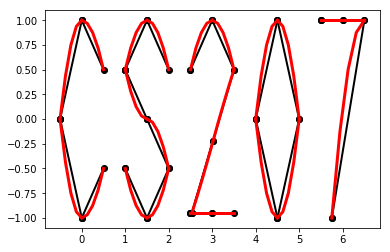
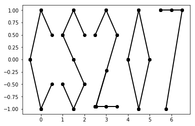
Drawing with Splines
DeriveAlive package as a surprise.- \(f_1(x) = \frac{-1}{0.5^2} x^2 + 1, x \in [-0.5, 0]\)
- \(f_2(x) = \frac{1}{0.5^2} x^2 - 1, x \in [-0.5, 0]\)
- \(f_3(x) = \frac{-1}{0.5} x^2 + 1, x \in [0, 0.5]\)
- \(f_4(x) = \frac{1}{0.5} x^2 - 1, x \in [0, 0.5]\)
- \(f_6(x) = \frac{-1}{0.5} (x-1.5)^2 + 1, x \in [1, 1.5]\)
- \(f_7(x) = \frac{1}{0.5} (x-1.5)^2 - 1, x \in [1, 1.5]\)
- \(f_8(x) = \frac{-1}{0.5} (x-1.5)^2, x \in [1.5, 2]\)
- \(f_9(x) = \frac{-1}{0.5} (x-1.5)^2 + 1, x \in [1.5, 2]\)
- \(f_{10}(x) = \frac{1}{0.5} (x-1.5)^2 - 1, x \in [1.5, 2]\)
- \(f_{11}(x) = \frac{-1}{0.5} (x-3)^2 + 1, x \in [2.5, 3]\)
- \(f_{12}(x) = \frac{-1}{0.5} (x-3)^2 + 1, x \in [3, 3.5]\)
- \(f_{13}(x) = 1.5x - 4.75, x \in [2.5, 3.5]\)
- \(f_{14}(x) = -1, x \in [2.5, 3.5]\)
- \(f_{15}(x) = \frac{-1}{0.5^2} (x-4.5)^2 + 1, x \in [4, 4.5]\)
- \(f_{16}(x) = \frac{1}{0.5^2} (x-4.5)^2 - 1, x \in [4, 4.5]\)
- \(f_{17}(x) = \frac{-1}{0.5^2} (x-4.5)^2 + 1, x \in [4, 4.5]\)
- \(f_{18}(x) = \frac{1}{0.5^2} (x-4.5)^2 - 1, x \in [4.5, 5]\)
- \(f_{19}(x) = 1, x \in [5.5, 6.5]\)
- \(f_{20}(x) = \frac{-1}{(-0.75)^2} (x-6.5)^2 + 1, x \in [5.75, 6.5]\)
>>> import surprise
# We first draw out the start and end points of each function
>>> surprise.drawPoints()
# Then we use the spline suite to draw quadratic splines based on the two points
>>> surprise.drawSpline()
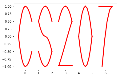
>>> surprise.drawTogether()